band_structure_of_nanocrystals
This is an old revision of the document!
Table of Contents
Band structure of nanocrystals
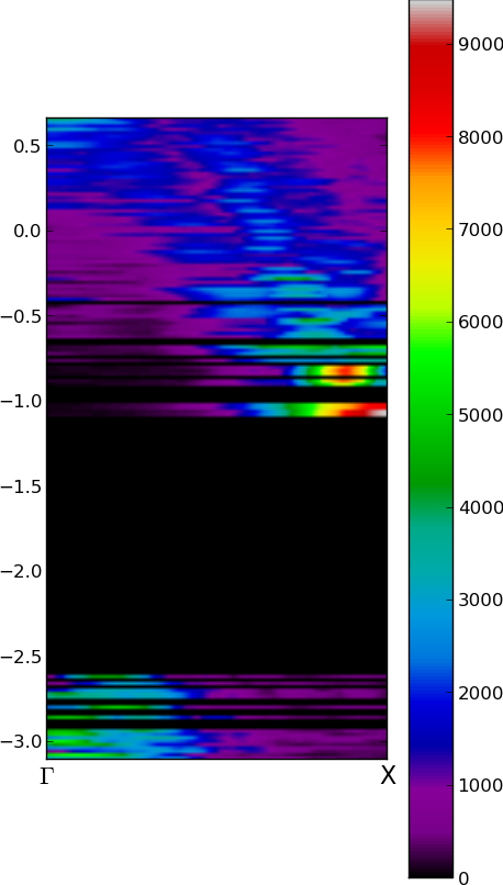
The 'fuzzy band structure' (i.e. cluster without periodic boundary condition) of an nanocrystal can be obtained by Fourier transform of it's eigenstates. See Hapala et.al,Phys.Rev.B87,195420. In fireball there are two methods to do this projection.
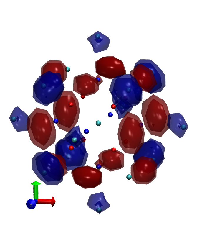
- 3D Fourier transform of molecular orbitals - in this method we choose several molecular orbitals, project them on grid and let fireball execute Fast fourier transform on this grid. The problem is that the result is complex ( real part correspond to symmetric components of the real wavefunction and imaginary part to antisymetric componenets ). For easier visualization we compute square of absolute value, which corresponds to density of the state in k-space. This property is exported as .xsf file.
Availability
this is implemented only in Prokop's personal versions of Fireball located in
/data/home/hapala/Fireball_dev/src_1.0-BSfinal
/data/home/hapala/Fireball_dev/progs_Jellium_mod
3D Fourier fransform of Molecular Orbitals
fireball.in
&OPTION
basisfile  = answer.bas
nstepf     = 1
icluster   = 1
ifixcharge = 1
dt         = 0.5
&END
&OUTPUT
iwrtewf     = 1
&END
&MESH
iewform = 5
npbands = 5
pbands = 159,160,161,162,163
&END
kmap.optional
1                  # byEnerg   - if 1 choose orbitals by energy range else choose by pbands list
-8.59705   1.09186 # Emin Emax - energy range
0                  # PlotXSF?  - save .xsf files
0                  # PlotPPN?  - save 2D projectins (max along z-axis) into ppn image file for quick overview
0                  # PlotImag? - save real and imaginery part to independent files  fft_Im_XXXX.xsf and fft_Re_XXXX.xsf
1                  # GetMaxPos - if 1 for each MO writes out position of global maximum of k-space density int kmaxs.dat
5.50               # alat      - lattice constant in angstroem
0                  # ValIn     - write out value in different points defined in ksamples.optional
ksample.optional
  26                  nksamples
  2.0  0.0  0.0   # HOMOs Gamma 100
  0.0  2.0  0.0
  0.0  0.0  2.0
 -2.0  0.0  0.0
  0.0 -2.0  0.0
  0.0  0.0 -2.0
  1.0  1.0  1.0   # HOMOs Gamma 111
 -1.0  1.0  1.0
  1.0 -1.0  1.0
 -1.0 -1.0  1.0
  1.0  1.0 -1.0
 -1.0  1.0 -1.0
  1.0 -1.0 -1.0
 -1.0 -1.0 -1.0
  0.0  1.0  1.0   # LUMOs   X
  0.0 -1.0  1.0
  0.0  1.0 -1.0
  0.0 -1.0 -1.0
  1.0  0.0  1.0
 -1.0  0.0  1.0
  1.0  0.0 -1.0
 -1.0  0.0 -1.0
  1.0  1.0  0.0
 -1.0  1.0  0.0
  1.0 -1.0  0.0
 -1.0 -1.0  0.0
kmaxs.dat
 iband, eigen_k(iband,1),   imax,    jmax,     kmax, ValMax,              rimax,          rjmax,        rkmax
 107     -7.40951516        -3        -3        -3   2968.71621697     -0.70854607     -0.70769619     -0.70733483
 108     -7.38731466        -4        -3        -2   3133.46757266     -0.94472810     -0.70769619     -0.47155655
 109     -7.38677828        -4        -2        -3   3128.34104148     -0.94472810     -0.47179746     -0.70733483
 110     -7.26838823        -4        -4         0   1878.06049291     -0.94472810     -0.94359492      0.00000000
 ...
ksamples.dat
  Ei         rho(k1)          rho(k2)        rho(k3)         rho(k4)          rho(k5)        rho(k6)
-2.08815     16.68657904      3.16266264     10.09450414     16.68657904      3.16266264     10.09450414     ...
-2.08681      5.87885299     17.02497532     10.22090870      5.87885299     17.02497532     10.22090870     ...
-2.06449     28.89941918     27.76432636     29.01794378     28.89941918     27.76432636     29.01794378     ...
...
1D cuts of Fuzzy Band Structure
fireball.in
&OPTION
basisfile  = answer.bas
nstepf     = 1
icluster   = 1
ifixcharge = 1
dt         = 0.5
&END
&OUTPUT
iwrtewf     = 1
&END
&MESH
iewform = 6
&END
kscan.optional
1                                # byEnerg
-8.0000  1.0000               # Emin Emax
5.50                             # alat
48   100                         # nlines nkpoints
2.0  0.0  0.0   1.0  1.0  0.0
2.0  0.0  0.0   1.0 -1.0  0.0
2.0  0.0  0.0   1.0  0.0  1.0
2.0  0.0  0.0   1.0  0.0 -1.0
0.0  2.0  0.0   1.0  1.0  0.0
0.0  2.0  0.0  -1.0  1.0  0.0
0.0  2.0  0.0   0.0  1.0  1.0
0.0  2.0  0.0   0.0  1.0 -1.0
0.0  0.0  2.0  -1.0  0.0  1.0
0.0  0.0  2.0   1.0  0.0  1.0
0.0  0.0  2.0   0.0  1.0  1.0
0.0  0.0  2.0   0.0 -1.0  1.0
-2.0  0.0  0.0  -1.0  1.0  0.0
-2.0  0.0  0.0  -1.0 -1.0  0.0
-2.0  0.0  0.0  -1.0  0.0  1.0
-2.0  0.0  0.0  -1.0  0.0 -1.0
0.0 -2.0  0.0   1.0 -1.0  0.0
0.0 -2.0  0.0  -1.0 -1.0  0.0
0.0 -2.0  0.0   0.0 -1.0  1.0
0.0 -2.0  0.0   0.0 -1.0 -1.0
0.0  0.0 -2.0   1.0  0.0 -1.0
0.0  0.0 -2.0  -1.0  0.0 -1.0
0.0  0.0 -2.0   0.0  1.0 -1.0
0.0  0.0 -2.0   0.0 -1.0 -1.0
1.0  1.0  1.0    0.0  1.0  1.0
1.0  1.0  1.0    1.0  0.0  1.0
1.0  1.0  1.0    1.0  1.0  0.0
-1.0  1.0  1.0    0.0  1.0  1.0
-1.0  1.0  1.0   -1.0  0.0  1.0
-1.0  1.0  1.0   -1.0  1.0  0.0
1.0 -1.0  1.0    0.0 -1.0  1.0
1.0 -1.0  1.0    1.0  0.0  1.0
1.0 -1.0  1.0    1.0 -1.0  0.0
-1.0 -1.0  1.0    0.0 -1.0  1.0
-1.0 -1.0  1.0   -1.0  0.0  1.0
-1.0 -1.0  1.0   -1.0 -1.0  0.0
1.0  1.0 -1.0    0.0  1.0 -1.0
1.0  1.0 -1.0    1.0  0.0 -1.0
1.0  1.0 -1.0    1.0  1.0  0.0
-1.0  1.0 -1.0    0.0  1.0 -1.0
-1.0  1.0 -1.0   -1.0  0.0 -1.0
-1.0  1.0 -1.0   -1.0  1.0  0.0
1.0 -1.0 -1.0    0.0 -1.0 -1.0
1.0 -1.0 -1.0    1.0  0.0 -1.0
1.0 -1.0 -1.0    1.0 -1.0  0.0
-1.0 -1.0 -1.0    0.0 -1.0 -1.0
-1.0 -1.0 -1.0   -1.0  0.0 -1.0
-1.0 -1.0 -1.0   -1.0 -1.0  0.0
klines_XXXXX.dat
       1    391.30476603    391.30476603    391.30476603    391.30476603    287.45162513  ...
       2    391.20959758    391.21921233    390.08793464    391.61800721    295.99428664  ...
       3    389.17880205    389.77130848    387.81208053    388.10778349    306.53352273  ...
       ...
klines_TOT.dat
Ei          rho(k1)         rho(k2)         rho(k3)         rho(k4)         rho(k5)       ...
-7.99755    413.91048549    428.76133304    440.87314746    450.14882297    456.52837031  ...
-7.99140    394.18797633    403.02567283    409.86012222    414.38007661    416.29758353  ...
-7.97472    418.51477832    433.83793597    448.50901654    462.18377663    474.53904963  ...
-7.96729    262.72449682    269.69434762    274.26597685    275.89514172    285.23659456  ...
...
plotting results
#!/usr/bin/python
from pylab import *
import numpy
dE    = 0.02             # [ eV ]choose width of energy-bins for plotting
F = transpose(genfromtxt( 'klines_TOT.dat' ))
Es = F[0]
Ps = transpose(F[1:])
Emin =Es.min(); Emax =Es.max()
Pgrid = zeros( ( int( (Emax-Emin)/dE )+1 ,  shape(Ps)[1] ) )
n = len(Es)
for i in range(n):
	iE = int((Es[i]-Emin)/dE)
	#Pgrid[iE] += Ps[i] 					      # overlaping (=degenerated) states are summed up
	Pgrid[iE] = numpy.vstack([Pgrid[iE],Ps[i] ]).max(axis=0)      # for overlaping (=degenerated) states is taken maximum
# choose color map reference here http://wiki.scipy.org/Cookbook/Matplotlib/Show_colormaps
cmap='spectral'
figure( figsize=(5,10) )
extent = ( 0,2, Emin, Emax )
imshow( Pgrid, origin='image', extent=extent, cmap = cmap )
xticks([0,2] , ['$\Gamma$','X'], fontsize=16)        # x-axis ticks Gamma and X vector
colorbar()
savefig('FuzzyBand.png',   bbox_inches='tight' )
show()
band_structure_of_nanocrystals.1416317631.txt.gz · Last modified: 2014/11/18 14:33 (external edit)


