Nanosurf Lab

To obtain the band structure of Si bulk of given lattice parameter we have to perform two steps. First, we need to achieve SCF solution. Therefore, we run a standard bulk calculation as described in the previous chapter. Let's calculate the band structure for the lattice parameter alat = 5.5 Å, than we have the fireball.in file containing:

&OPTION
basisfile = Si.bas
lvsfile = Si.lvs
kptpreference = Si.kpts
nstepf = 1
rescal = 5.5
&END

where Si.bas, Si.lvs and Si.kpts files are identical as those used in previous chapter. Once we obtain the SCF solution, we can determine the Fermi level from an output file:

mac135> grep "Fermi Level" $output_file | tail -1
 Fermi Level =   -4.33045968490834 

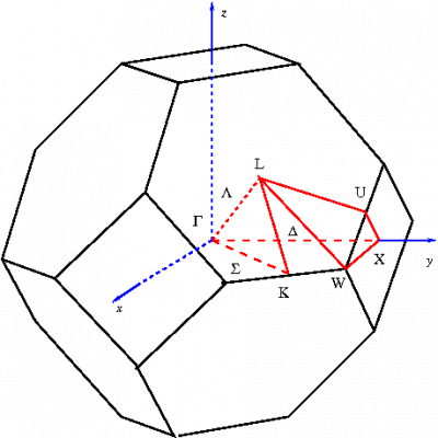
In next step, we run the FIREBALL code again, but now with fixed charges (ifixcharge = 1) and with a new set of k-points in desired high-symmetry directions in the first Brillouin zone. Remember we need having CHARGES file in a working directory for a restart. In this particular case,we have chosen a direction L-Γ-X-Γ stored in a lgxg.kpts file (see also fig. 1).

In addition, we have to write out a list of eigenvalues at each k-point switching on iwrteigen variable. Our input file fireball.in has following form now:

&OPTION
basisfile = Si.bas
lvsfile = Si.lvs
kptpreference = lgxg.kpts
nstepf = 1
ifixcharge = 1
rescal = 5.5
&END
&OUTPUT
iwrteigen = 1
&END

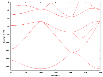
After the run, we obtain a file ek.dat appears in a working directory. This file contains at each line set of eigenvalues for given k-points ordered in ascending form. The Fermi level can Now we have all information to plot the band structure of the Si bulk.

mac135> gnuplot
gnuplot> set xrange [0:300]
gnuplot> set yrange [-17:0]
gnuplot> set xlabel "k-points"
gnuplot> set ylabel "Energy [eV]"
gnuplot> set nokey
gnuplot> set multiplot
multiplot> plot "ek.dat" using 1:2 with lines
multiplot> plot "ek.dat" using 1:3 with lines
multiplot> plot "ek.dat" using 1:4 with lines
multiplot> plot "ek.dat" using 1:5 with lines
multiplot> plot "ek.dat" using 1:6 with lines
multiplot> plot "ek.dat" using 1:7 with lines

To plot Density of state, first, we have to achieve SCF solution in the same way as above (see previous section). Next we perform calculation with fixed SCF charges (switching on ifixcharge =1). The DOS calculation is initialized via variable iwrtdos in the section &OUTPUT. Hence, our fireball.in file looks like that:

&OPTION
basisfile = Si.bas
lvsfile = Si.lvs
kptpreference = Si.kpts
nstepf = 1
ifixcharge = 1
rescal = 5.5
&END
&OUTPUT
iwrtdos = 1
&END

In addition, dos.optional has to be presented in a working directory having following distance:

1.0                   ! scale factor (leave 1.0)
1        2            ! list of atoms to analyze DOS
360                   ! number of energy steps
-18.0   0.05          ! initial energy, energy step 
0                     ! leave untouched
0.0     0.0           ! leave untouched
0.05                  ! imaginary part of Green function (controls energy level smearing) 

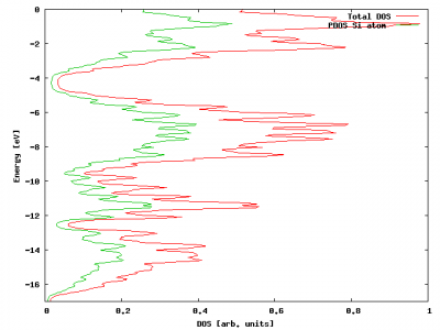
After finishing a run, we obtain dens_001.dat,dens_002.dat including projected DOS on two Si atoms in the unit cell (including projected DOS onto individual shells of atoms). Additionally, there is a file dens_TOT.dat containing DOS. Here, a first column means energy and a second one DOS.

mac135> gnuplot
gnuplot> set xrange [0:1]
gnuplot> set yrange [-17:0]
gnuplot> set xlabel "DOS [arb. units]"
gnuplot> set ylabel "Energy [eV]"
gnuplot>  plot "dens_TOT.dat" using 2:1 title 'Total DOS' with lines, \
          "dens_001.dat" using 11:1 title 'PDOS Si atom ' with lines

$ ls
Fdata  uno.bas  uno.kpts  uno.lvs  vol.sh

$ head uno.bas
2
14      0.000000      0.000000      0.000000
14      0.250000      0.250000      0.250000

$ head uno.kpts
32 
-2.35619449         -2.35619449         -2.35619449        0.03125000
-3.92699081         -0.78539816         -0.78539816        0.03125000
-5.49778713          0.78539816          0.78539816        0.03125000
-7.06858347          2.35619449          2.35619449        0.03125000
-0.78539816         -3.92699081         -0.78539816        0.03125000
-2.35619449         -2.35619449          0.78539816        0.03125000
-3.92699081         -0.78539816          2.35619449        0.03125000
-5.49778713          0.78539816          3.92699081        0.03125000
 0.78539816         -5.49778713          0.78539816        0.03125000 

$ head  uno.lvs
0.5000    0.5000    0.0000
0.5000    0.0000    0.5000
0.0000    0.5000    0.5000

The script to calculate the bulk modulus

$ cat vol.sh 
#!/bin/bash
 
##----- Parametros de control (el parametro de red tiene que encontrase entre ini fin  --------##
N=10
ini=5.0
fin=6.0 
 
##----------Funcion analisis para dos atomos/celda-----------------------------------------##
function analisis {
ETOT=$(grep 'ETOT' salida.out|cut -d'=' -f2)
sigma=$(grep sigma salida.out | cut -d'=' -f16 | tail -1)
charge=$(head -2 uno.bas | tail -1 | tr -s ' ' | cut -d' ' -f2)' -> '$(head -2 CHARGES | tail -1)
charge=$charge' ;'$(head -3 uno.bas | tail -1 | tr -s ' ' | cut -d' ' -f2)' -> '
charge=$charge$(tail -1 CHARGES)
echo $rescal$'\t'$ETOT$'\t'$sigma$'\t'$charge$'\t'>>salida
}
##------------------------------------------------------------------------------------------##
function start {
rm -fr salida
for((i=0;i<=N;i++))
do
rescal=$(python -c "print '%.6f' % ($i*1.0*($fin-$ini)/$N+$ini)")
echo "&option
basisfile = uno.bas
lvsfile = uno.lvs
kptpreference = uno.kpts
rescal = $rescal
sigmatol = 0.000001
nstepf = 1
&end
&output
iwrtxyz = 1
&end" > fireball.in 
../progs/fireball.x > salida.out    

analisis
done
}
##----------------------------------1º start  ----------------------------------------------##
start
##-----------------------------buscamos el minimo ------------------------------------------##
min=$(python -c "
x0 = []
y0 = []
for line in file(\"salida\"):
   line = line.split()
   x = line[0]
   y = line[1]
   x0.append(x)
   y0.append(y)  

j=0
for i in range(len(x0)):
  if y0[j]< y0[i]:
    j=i
print x0[j]")
cp salida borrar
rm -fr aux.py		        

##----------------------------------2º start -----------------------------------------------##
N=40
d=0.4
ini=$(python -c "print '%.6f' % (1.0*($min-$d))")
fin=$(python -c "print '%.6f' % (1.0*($min+$d))")
start
mv salida Vol.dat
##------------------------------------------------------------------------------------------##  

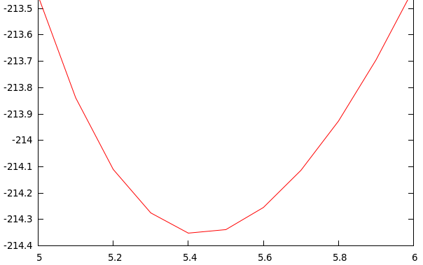
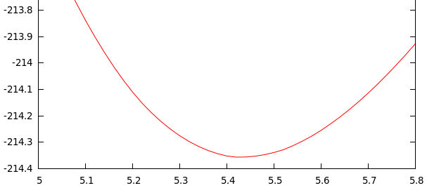
In the 1º start of the script “vol.sh” takes 10 points between 5-6:

In the 2º start of the script “vol.sh” takes 40 points between the minimum of the 1º start

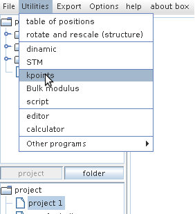
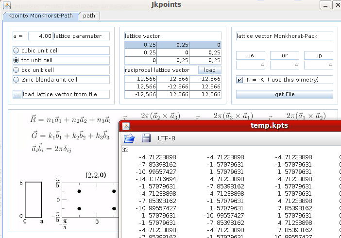
The scripts uses the parameter rescal in fireball.in and unitary positions and lattice vectors with 2 atoms/cell to obtain the kpts points we used xeo:

The bulk mudulus can be calculed also with xeo (Utilities→Bulk modulus), in the in line command:

$ xeo -Bulk Vol.dat zincblende
E_min =     -214.35239    eV
a_min =        5.43719    angs 
Volumen =       40.18518 ang**3 
Bulk modulus =      100.79399  GPa